Policy Gradient (PG)
Gaussian Policy Gradient (PG)에 대해서 알아 보고 Gym에서 제공하는 문제를 해결하기 위해 Policy-Network을 모델링 하고 최적의 액션을 예측하는 알고리듬을 만들어 보자.
실제로 돌려 보고 싶으면 구글 코랩으로 ~
![]()
문제 (Problem)
👤 보스
딥러닝의 출력을 Q-value로 하지 않고
액션(action)이 바로 나오도록 하면
더 깔끔할 것 같은데…아래 체육관(Gym)에 가서
‘달착륙선’ 문제를 내가 말한 방법으로 풀어 보게~
⚙️ 엔지니어
말은 쉽지…
문제 분석 (Problem Analysis)
‘달착륙선’을 동작 시키기 위해서는 Box2D를 설치해야 한다.
!pip install gym[box2d]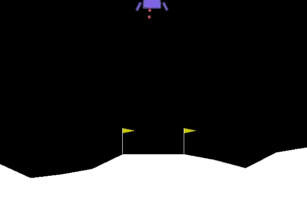
달 착륙선의 주 엔진과 오른쪽, 왼쪽에 있는 보조 엔진의 파워를 조종해서 깃발 사이로 안전하게 착륙 시키는 것이 목표다.
환경 (Environment)
‘달착륙선’ 의 환경은 8종류의 상태(State)와 2종류의 액션(Action)으로 구성 되어 있다.
import gym
import numpy as np

env = gym.make('LunarLanderContinuous-v2')

state = env.reset()
action = env.action_space.sample()

print('State space: ', env.observation_space)
print('Initial state: ', state)
print('\nAction space: ', env.action_space)
print('Random action: ', action)
State space: Box(8,)
Initial state: [ 0.00285416 1.4058137 0.28906897 -0.22695263 -0.00330036 -0.06547835
0. 0. ]
Action space: Box(2,)
Random action: [ 0.8797723 -0.36046624]
액션 (Action)
‘달착륙선’의 액션(action)은 2개의 실수값의 배열로 되어 있다.
\(A = \begin{bmatrix} \{ a_{00}, a_{01} \}, \\ \{ a_{10}, a_{11} \}, \\ \{ a_{20}, a_{21} \}, \\ \{ a_{30}, a_{31} \} \end{bmatrix}\)
| Index | State | Control |
|---|---|---|
| 0 | 주 엔진 | -1..0 off, 0..+1 throttle from 50% to 100% power |
| 1 | 왼쪽, 오른쪽 보조 엔진 | -1.0..-0.5 fire left engine, +0.5..+1.0 fire right engine, -0.5..0.5 off |
상태 (State)
‘달착륙선’의 상태(State) \(S\)는 8개의 실수값의 배열로 되어 있다.
\(S = \begin{bmatrix} \{ s_{00}, s_{01}, \cdots\}, \\ \{ s_{10}, s_{11}, \cdots \}, \\ \{ s_{20}, s_{21}, \cdots \}, \\ \{ s_{30}, s_{31}, \cdots \} \end{bmatrix}\)
| Index | State | Value |
|---|---|---|
| 0 | 달착륙선 X 좌표값 | -Inf ~ Inf |
| 1 | 달착륙선 Y 좌표값 | -Inf ~ Inf |
| 2 | 달착륙선 X축 속도 | -Inf ~ Inf |
| 3 | 달착륙선 Y축 속도 | -Inf ~ Inf |
| 4 | 달착륙선 각도 | -Inf ~ Inf |
| 5 | 달착륙선 각속도 | -Inf ~ Inf |
| 6 | 왼쪽 다리가 땅에 닿았나? | 1 (Yes), 0 (No) |
| 7 | 오른쪽 다리가 땅에 닿았나? | 1 (Yes), 0 (No) |
⚙️ 엔지니어
상태(State)의 개수는 무한대
액션(action)도 아날로그 이다!
보상 (Reward)
- Reward for moving from the top of the screen to landing pad and zero speed is about 100..140 points.
- If lander moves away from landing pad it loses reward back.
- Episode finishes if the lander crashes or comes to rest, receiving additional -100 or +100 points.
- Each leg ground contact is +10
- Firing main engine is -0.3 points each frame
- Firing side engine is -0.03 points each frame
- Solved is 200 points
⚙️ 엔지니어
상태(State), 액션(Action), 보상(Reward) 모두 복잡하다….
Gaussian Policy Gradient
우리의 목표는 상태(state) 데이터를 입력(\(s\))으로, 아날로그 액션(action)을 출력(\(\hat a\))으로 하는 뉴럴 네트워크를 구성하고 학습을 통해서 주어진 상태에서 최적의 액션을 예측하도록 하는 것이다.
가우시안 분포 (Gaussian Distribution)
PG를 모델링하기 위해서 아래 세가지를 전제로 한다.
- ‘달착륙선’을 안전하게 깃발 사이로 착륙 시키기 위한 최적의 액션값 \(a\) 들은 가우시안 분포(\(\mu, \sigma\))를 따른다.
- 우리가 설계할 뉴럴 네트워크 모델의 출력값 \(\hat y\) 은 액션에 대한 가우시안 분포의 평균값 \(\mu\) 이다.
- PG에서 뉴럴 네트워크의 파라미터는 \(w\)가 아닌 \(\theta\)로 표시한다.
예를 들어 보자.
슈퍼 마리오 브라더스 게임에서 마리오는 쿠파를 만나면 점프를 해서 피해야 한다.

이제 게임을 진행하면서 점프를 해서 쿠파를 피한 경우에 점프를 시작할 때의 마리오와 쿠파와의 거리 \(x\)를 적어 둔다.
하루 종일 게임을 하고 나서 점프에 성공한 횟수와 거리와의 관계를 그래프로 표시하면 다음과 같다.
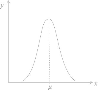
딱 봐도 가우시안 분포 곡선이다. 이 그래프가 말하고 있는 것은 마리오의 액션(점프)는 가우시안 분포를 따른다는 것이고, 가우시안 분포의 평균값 \(\mu\)에서 점프하는 것이 최적의 액션이라는 것이다.
⚙️ 엔지니어
뉴럴 네트워크의 입력 \(x\)는 상태(State), 출력 \(\hat y\)은 액션의 가우시안 분포의 평균값 \(\mu\)으로 설정하고
\(\mu\) 를 그 상태(State)에서의 최적의 액션값 \(a\) 에 근사하도록 최적화를 해주면 된다!그런데 손실함수는 어떻게 생겼지?
로그 라이클리후드 함수 (Log Likelihood Function)
가우시안 분포에서 주어진 데이터가 있을때에 \(\mu\)를 알아내기 위해서는 로그 라이클리후드 (Log Likelihood) 함수를 사용한다.
\(\theta\)의 조건에 따른 n개의 액션 데이터 \(a\) 가 주어졌을때 액션의 \(\mu\)값은 아래 식을 가지고 계산할 수 있다.
\(\begin{align} \log p(a ; \theta) & = \log l(\theta ; a) \\ & = \sum_{i=1}^n \left( -\dfrac{(a_i -\mu_{\theta})^2}{2\sigma^2} - \dfrac{1}{2}\log{\sigma^2} -\dfrac{1}{2}\log(2\pi)\right) \end{align}\)
여기서는 로그 라이클리후드의 ‘최대값’을 찾아야 한다. 왜냐하면 \(\mu\) 에 대한 \(p(a ; \theta)\) 가 최대값이 되어야 하기 때문이다. 최대값을 찾는 방법을 경사 상승법 (Gradient Ascent)이라고 한다.
경사 상승법 (Gradient Ascent)
경사 하강법의 반대다. 등산을 잘 하게 해서 산꼭대기에 오르게 하는 것이다.
로그 라이클리 후드 함수를 \(\theta\)에 대해서 미분을 하고 그 값을 \(\theta\)에 업데이트를 하면 \(\hat \mu\)값을 얻을 수 있다.
\(\begin{align} & \dfrac{\partial \log p(a ; \theta)}{\partial \theta} = \nabla_{\theta} \log p(a ; \theta) \\ \\ & \theta \leftarrow \theta + \alpha \nabla_{\theta} \log p(a ; \theta) \end{align}\)
⚙️ 엔지니어
그러나
이것은 최적의 \(\hat \mu\)가 아니다!
왜냐하면
액션 a가 ‘최적의 액션’인지 최악의 액션인지 모른다.
최적의 액션은 돌아올 보상이 큰 액션이다!
뭔가 추가적으로 보상과 관련된 함수가 필요하다
그것은 바로…
어드밴티지 함수 (Advantage Function)
아이디어는 단순하다. 돌아올 보상이 큰 액션에 대해서는 등산을 잘 하게 하고, 돌아올 보상이 작거나 마이너스인 액션에 대해서는 등산을 못하게 하는 것이다. 어드밴티지 함수는 ‘표준화’를 잘 시켜 주어야 한다. 1을 넘어가는 경우에는 산꼭대기를 지나칠 수 있기 때문이다. 평균을 0으로 표준편차를 1로 표준화를 해 준다.
\(\begin{align} & f(s) : \text{advantage function} \\ & \theta \leftarrow \theta + \alpha \nabla_{\theta} \log p(a ; \theta) f(s) \end{align}\)
돌아올 보상에 대한 어드벤티지 함수는 어떤 가치(Value)와 알고리듬을 사용하는지에 따라 아래와 같이 나눌 수 있다.
State-value를 사용하는 방법 (REINFORCE)
\(f(s) = G_t - \hat v(s, w)\)Q-value 를 사용하는 방법 (Q Actor-Critic)
\(f(s) = q(s,a) - \hat q(s,a,w)\)Q-value와 State-value를 사용하는 방법 (Advantage Actor-Critic)
\(f(s) = q(s, a) - \hat v(s,w)\)TD를 사용하는 방법 (TD Actor-Critic)
\(f(s) = r + \gamma v(s’) - \hat v(s, w)\)
여기서는 가장 간단한 REINFORCE 방법을 사용한다.
Policy Grdient 모델링 (Modeling)
Policy-Network 모델링과 상태가치(State-value) 모델링 두개를 모델링 해야 한다.
Policy-Network 모델링 (Modeling)
상태(state)와 어드벤티지(state-value)를 데이터를 입력(\(s\))으로, 액션(action)의 평균을 출력(\(\hat \mu\))으로 하는 뉴럴 네트워크를 구성한다.
데이터 수집
입력 데이터 \(X\)는 상태(State), \(Y\)는 액션(action)이다.
\(\begin{align} & X = \{ s_1^{(i)}, s_2^{(i)}, s_3^{(i)}, s_4^{(i)}, s_5^{(i)}, s_6^{(i)}, s_7^{(i)}, s_8^{(i)} \} \\ & s_1^{(i)} : \text{i 번째 달착륙선 X 좌표값} \\ & s_2^{(i)} : \text{i 번째 달착륙선 Y 좌표값} \\ & s_3^{(i)} : \text{i 번째 달착륙선 X축 속도} \\ & s_4^{(i)} : \text{i 번째 달착륙선 Y축 속도} \\ & s_5^{(i)} : \text{i 번째 달착륙선 각도} \\ & s_6^{(i)} : \text{i 번째 달착륙선 각속도} \\ & s_7^{(i)} : \text{i 번째 왼쪽 다리가 땅에 닿았나?} \\ & s_8^{(i)} : \text{i 번째 오른쪽 다리가 땅에 닿았나?} \\ \\ & Y = \{a_1^{(i)}, a_2^{(i)})\} \\ & a_1^{(i)} : \text{주 엔진 파워 값} \\ & a_2^{(i)} : \text{왼쪽, 오른쪽 보조 엔진 파워 값} \end{align}\)
모델링
\(\begin{align} & \hat Y = \{ \hat a_1^{(i)}, \hat a_2^{(i)} \} \\ & \hat a_1^{(i)} = \hat \mu_1 (s, \theta) \\ & \hat a_2^{(i)} = \hat \mu_2 (s, \theta) \end{align}\)
손실 함수 (Loss function)
손실함수는 로그 라이클리후드 함수와 어드벤티지 함수를 곱한 것의 평균(기대값)에다가 경사를 하강하기 위해서 마이너스를 붙여 준다.
\(J(\theta) = - \dfrac{1}{N} \sum_{i=1}^N \nabla_{\theta} \log p(a ; \theta) * \hat A_{\text{std}}\)
손실함수 \(J(\theta)\) 는 Keras에서 API를 제공하지 않는다. 따라서 Tensorflow를 이용해서 직접 만들어야 한다. Tensorflow는 Graph와 Session에 대한 개념을 알고 있으면 쉽게 사용할 수 있다.
경사 하강법 (Gradient Descent)
Tensorflow의 Optimizer는 경사 하강 방식이다. 우리는 간단하게 손실 함수에 마이너스(-)를 붙여 줌으로써 경사 하강법을 사용할 수 있다.
REPEAT(epoch) {
\(\theta \leftarrow \theta-\alpha \dfrac{\partial J(\theta)}{\partial \theta}\)
}
\(\alpha\): learining rate
로그 표준편차 (Log standard deviation)
로그 표준편차(logstd)를 tf.variable로 선언한다. 손실을 최적화 하면서 로그 표준편차 값도 최적화 된다.
샘플 액션 (Sampled Action)
평균의 ±1 표준편차 안에서 랜덤하게 액션을 선택한다.
import tensorflow as tf
from tensorflow.keras.layers import Dense

# Input Dimensions
states_dim = env.observation_space.shape[0]
action_dim = env.action_space.shape[0]

# Placeholders for inputs.
input_state = tf.placeholder(shape=[None, states_dim], name="state", dtype=tf.float32)
input_action = tf.placeholder(shape=[None, action_dim], name="action", dtype=tf.float32)
input_advan = tf.placeholder(shape=[None], name="advan", dtype=tf.float32)
n = tf.shape(input_state)[0]

# The log std vector, it's a parameter.
logstd = tf.get_variable("logstd", shape=[action_dim], initializer=tf.zeros_initializer())
logstd_n = tf.ones(shape=(n, action_dim), dtype=tf.float32) * logstd

# The policy network.
hidden1 = Dense(32, activation='relu')(input_state)
hidden2 = Dense(32, activation='relu')(hidden1)
mean = Dense(action_dim, activation=None)(hidden2)

# Computing the log likelihood.
variance = tf.exp(2*logstd_n)
func = -tf.square(input_action - mean)/(2*variance) - 0.5*tf.log(tf.constant(2*np.pi)) - logstd_n
log_likelihood = tf.reduce_sum(func, axis=[1])

# Diagonal Gaussian distribution for sampling actions
sampled_action = (tf.random_normal(tf.shape(mean)) * tf.exp(logstd_n) + mean)[0]

# Loss function
loss_op = - tf.reduce_mean(log_likelihood * input_advan)
# Optimizer
update = tf.train.AdamOptimizer().minimize(loss_op)
WARNING: Logging before flag parsing goes to stderr.
W1011 14:45:44.354567 140289627080512 deprecation.py:506] From /home/dataman/anaconda3/lib/python3.7/site-packages/tensorflow/python/ops/init_ops.py:1251: calling VarianceScaling.__init__ (from tensorflow.python.ops.init_ops) with dtype is deprecated and will be removed in a future version.
Instructions for updating:
Call initializer instance with the dtype argument instead of passing it to the constructor
상태가치 모델링 (State-Value Modeling)
상태(State)의 개수가 무한대이기 때문에 뉴럴 네트워크를 이용해서 상태 가치(State Value)를 예측 해야 하지만 귀찮다. 여기서는 간단하게 선형 회귀 (Linear Regression)을 이용한다.
데이터 수집 (Data Collection)
입력 데이터 \(X\)는 상태(State), \(Y\)는 돌아올 보상, 리턴 \(G_t\)이다.
\(\begin{align} & X = \{ s_1^{(i)}, s_2^{(i)}, s_3^{(i)}, s_4^{(i)}, s_5^{(i)}, s_6^{(i)}, s_7^{(i)}, s_8^{(i)}\} \\ & s_1^{(i)} : \text{i 번째 달착륙선 X 좌표값} \\ & s_2^{(i)} : \text{i 번째 달착륙선 Y 좌표값} \\ & s_3^{(i)} : \text{i 번째 달착륙선 X축 속도} \\ & s_4^{(i)} : \text{i 번째 달착륙선 Y축 속도} \\ & s_5^{(i)} : \text{i 번째 달착륙선 각도} \\ & s_6^{(i)} : \text{i 번째 달착륙선 각속도} \\ & s_7^{(i)} : \text{i 번째 왼쪽 다리가 땅에 닿았나?} \\ & s_8^{(i)} : \text{i 번째 오른쪽 다리가 땅에 닿았나?} \\ \\ & Y = v^{(i)} = G^{(i)}_t, \quad \text{i 번째 리턴값} \end{align}\)
모델링(Modeling)
\(\hat Y = \hat v^{(i)} = w^T X + b \)
손실함수(Loss Function)
몬테 카를로 방식으로 돌아다니면서 얻은 보상의 리턴 값 \(G_t\) 과 선형 회귀에서 얻은 가치 값 \(\hat v\) 과의 평균 제곱 오차(Mean-squared error)를 손실 함수로 정의한다.
\({\large J}(w, b) = \dfrac{1}{2m} \sum_{i=1}^m (G_t^{(i)} - \hat v^{(i)} (S, w, b))^2\)
경사 하강법(Gradient Descent)
REPEAT(epoch) {
\(\begin{align}
w & \leftarrow w-\alpha \dfrac{\partial J(w,b)}{\partial w} \\
b & \leftarrow b-\alpha \dfrac{\partial J(w,b)}{\partial b}
\end{align}\)
}
\(\alpha\): learining rate
from sklearn.linear_model import LinearRegression
# State-value function approximator
approx = LinearRegression()
# Initialization
approx.fit(np.array([0]*states_dim).reshape((1,states_dim)), np.array([0]).reshape((1,1)))
LinearRegression(copy_X=True, fit_intercept=True, n_jobs=None, normalize=False)
에이전트 (Agent)
평균의 ±1 표준편차 안에서 랜덤하게 액션을 수행 하면서 데이터를 수집하고 최적의 액션으로 업데이트 한다.
메모리 (Memory)
min_timesteps_per_batch 만큼 액션을 수행한 결과(state, action, reward)를 저장한다.
리플레이 (Replay)
저장된 데이터들을 상태가치(state-value) 모델에 넣고 훈련한다. 그리고 Policy-Network 모델에 넣고 훈련한다.
학습 (Learning)
돌려 놓고 커피 한잔 하세여~ ☕️
def predict(sess, state):
    with sess.as_default():
        action = sess.run(sampled_action, feed_dict={input_state: state[None]})
    return action

def fit(sess, state, action, advantage):
    with sess.as_default():
        sess.run([update], feed_dict={input_state: state, input_action: action, input_advan: advantage})
import scipy.signal
def get_returns(x, gamma):
return scipy.signal.lfilter([1],[1,-gamma],x[::-1], axis=0)[::-1]from tqdm import tqdm
from tensorflow.keras import backend as K
sess = tf.Session()
K.set_session(sess)
sess.run(tf.global_variables_initializer())
num_iteration = 500
gamma = 0.97
min_timesteps_per_batch = 3000
total_timesteps = 0
for i in tqdm(range(num_iteration)):
timesteps_this_batch = 0
memory = []
while True:
state = env.reset()
states, actions, rewards = [], [], []
while True:
states.append(state)
action = predict(sess, state)
actions.append(action)
state, reward, done, _ = env.step(action)
rewards.append(reward)
if done:
break
# Memory
path = {"state" : np.array(states), "action" : np.array(actions), "reward" : np.array(rewards)}
memory.append(path)
timesteps_this_batch += len(path["reward"])
if timesteps_this_batch > min_timesteps_per_batch:
break
total_timesteps += timesteps_this_batch
# Replay
# Advantage function
G_ts, advs = [], []
for path in memory:
rew_t = path["reward"]
G_t = get_returns(rew_t, gamma)
v_hat = approx.predict(path["state"])
adv = G_t - v_hat.flatten()
advs.append(adv)
G_ts.append(G_t)
# Build data set
in_states = np.concatenate([path["state"] for path in memory])
in_actions = np.concatenate([path["action"] for path in memory])
advans = np.concatenate(advs)
in_advans = (advans - advans.mean()) / (advans.std() + 1e-8)
G_ts = np.concatenate(G_ts)
# Update State-value
approx.fit(in_states, G_ts)
# Update Policy
fit(sess, in_states, in_actions, in_advans)100%|██████████| 500/500 [47:44<00:00, 8.59s/it]
해결 (Solution)
달착륙선을 인공지능이 조종해서 무사히 착륙하고 있다!
from gym.wrappers import Monitor

import base64
from IPython.display import HTML
from IPython import display as ipythondisplay

from pyvirtualdisplay import Display
display = Display(visible=0, size=(1400, 900))
display.start()

def show_video(file_infix):
    with open('./video/openaigym.video.%s.video000000.mp4' % file_infix, 'r+b') as f:
        video = f.read()
        encoded = base64.b64encode(video)
        ipythondisplay.display(HTML(data='''<video alt="Trained CartPole" autoplay
                loop style="height: 200px;">
                <source src="data:video/mp4;base64,{0}" type="video/mp4" />
                 </video>'''.format(encoded.decode('ascii'))))

def wrap_env(env):
    env = Monitor(env, './video', force=True)
    return env
W1011 15:35:43.337823 140289627080512 abstractdisplay.py:151] xdpyinfo was not found, X start can not be checked! Please install xdpyinfo!
import gym
import numpy as np

#num_state = env.observation_space.shape[0]
#num_action = env.action_space.shape[0]

env = wrap_env(gym.make('LunarLanderContinuous-v2'))
state = env.reset()
done = False

while not done:
    action = predict(sess, state)
    state, reward, done, info = env.step(action)

file_infix = env.file_infix
env.close()

show_video(file_infix)- 참고한 코드는 아래와 같다.
https://github.com/DanielTakeshi/rl_algorithms/tree/master/vpg